


Time Series Analysis in Python
Learn how to estimate, forecast, and simulate these models using statistical libraries in Python. You'll see numerous examples of how these models are used, with a particular emphasis on applications in finance.
From stock prices to climate data, time series data are found in a wide variety of domains, and being able to effectively work with such data is an increasingly important skill for data scientists. This course will introduce you to time series analysis in Python. After learning about what a time series is, you'll learn about several time series models ranging from autoregressive and moving average models to cointegration models. Along the way, you'll learn how to estimate, forecast, and simulate these models using statistical libraries in Python. You'll see numerous examples of how these models are used, with a particular emphasis on applications in finance.
Download Datasets and Presentation slides for this post HERE
This post is 2nd part of Time Series with Python Track from DataCamp. The track includes:
import pandas as pd
import numpy as np
import warnings
import matplotlib.pyplot as plt
import matplotlib as mpl
mpl.rcParams['figure.dpi'] = 150
pd.set_option('display.expand_frame_repr', False)
plt.style.use('ggplot')
mpl.rcParams['figure.figsize'] = (15, 15)
mpl.rcParams['axes.grid'] = True
warnings.filterwarnings("ignore")
Correlation and Autocorrelation
In this chapter you'll be introduced to the ideas of correlation and autocorrelation for time series. Correlation describes the relationship between two time series and autocorrelation describes the relationship of a time series with its past values.
Introduction to Course
A "Thin" Application of Time Series
Google Trends allows users to see how often a term is searched for. We downloaded a file from Google Trends containing the frequency over time for the search word "diet", which is pre-loaded in a DataFrame called diet. A first step when analyzing a time series is to visualize the data with a plot. You should be able to clearly see a gradual decrease in searches for "diet" throughout the calendar year, hitting a low around the December holidays, followed by a spike in searches around the new year as people make New Year's resolutions to lose weight.
Like many time series datasets you will be working with, the index of dates are strings and should be converted to a datetime index before plotting.
Instructions:
- Convert the date index to datetime using pandas's to_datetime().
diet = pd.read_csv('./datasets/diet.csv', index_col=0)
diet.head()
diet.index = pd.to_datetime(diet.index)
- Plot the time series and set the argument grid to True to better see the year-ends.
diet.plot(grid=True)
plt.show()

- Slice the diet dataset to keep only values from 2012, assigning to diet2012.
- Plot the diet2012, again creating gridlines with the grid argument.
diet.index = pd.to_datetime(diet.index)
# Slice the dataset to keep only 2012
diet2012 = diet[diet.index.year == 2012]
# Plot 2012 data
diet2012.plot(grid=True)
plt.show()

Notice how searches for 'diet' spiked up after the holidays every year.
Merging Time Series With Different Dates
Stock and bond markets in the U.S. are closed on different days. For example, although the bond market is closed on Columbus Day (around Oct 12) and Veterans Day (around Nov 11), the stock market is open on those days. One way to see the dates that the stock market is open and the bond market is closed is to convert both indexes of dates into sets and take the difference in sets.
The pandas .join() method is a convenient tool to merge the stock and bond DataFrames on dates when both markets are open.
Stock prices and 10-year US Government bond yields, which were downloaded from FRED, are pre-loaded in DataFrames stocks and bonds.
Instructions:
- Convert the dates in the stocks.index and bonds.index into sets.
- Take the difference of the stock set minus the bond set to get those dates where the stock market has data but the bond market does not.
- Merge the two DataFrames into a new DataFrame, stocks_and_bonds using the .join() method, which has the syntax df1.join(df2).
- To get the intersection of dates, use the argument how='inner'.
stocks = pd.read_csv('./datasets/stocks.csv', index_col=0)
bonds = pd.read_csv('./datasets/bonds.csv', index_col=0)
import pandas as pd
# Convert the stock index and bond index into sets
set_stock_dates = set(stocks.index)
set_bond_dates = set(bonds.index)
# Take the difference between the sets and print
print(set_stock_dates - set_bond_dates)
# Merge stocks and bonds DataFrames using join()
stocks_and_bonds = stocks.join(bonds, how='inner')
Pandas helps make many time series tasks quick and efficient.
Correlation of Stocks and Bonds
Investors are often interested in the correlation between the returns of two different assets for asset allocation and hedging purposes. In this exercise, you'll try to answer the question of whether stocks are positively or negatively correlated with bonds. Scatter plots are also useful for visualizing the correlation between the two variables.
Keep in mind that you should compute the correlations on the percentage changes rather than the levels.
Stock prices and 10-year bond yields are combined in a DataFrame called stocks_and_bonds under columns SP500 and US10Y
The pandas and plotting modules have already been imported for you. For the remainder of the course, pandas is imported as pd and matplotlib.pyplot is imported as plt.
Instructions:
- Compute percent changes on the stocks_and_bonds DataFrame using the .pct_change() method and call the new DataFrame returns.
- Compute the correlation of the columns SP500 and US10Y in the returns DataFrame using the .corr() method for Series which has the syntax series1.corr(series2).
- Show a scatter plot of the percentage change in stock and bond yields.
returns = stocks_and_bonds.pct_change()
# Compute correlation using corr()
correlation = returns['SP500'].corr(returns['US10Y'])
print("Correlation of stocks and interest rates: ", correlation)
# Make scatter plot
plt.scatter(returns['SP500'],returns['US10Y'])
plt.show()

The positive correlation means that when interest rates go down, stock prices go down. For example, during crises like 9/11, investors sold stocks and moved their money to less risky bonds (this is sometimes referred to as a 'flight to quality'). During these periods, stocks drop and interest rates drop as well. Of course, there are times when the opposite relationship holds too.
Flying Saucers Aren't Correlated to Flying Markets
Two trending series may show a strong correlation even if they are completely unrelated. This is referred to as "spurious correlation". That's why when you look at the correlation of say, two stocks, you should look at the correlation of their returns and not their levels.
To illustrate this point, calculate the correlation between the levels of the stock market and the annual sightings of UFOs. Both of those time series have trended up over the last several decades, and the correlation of their levels is very high. Then calculate the correlation of their percent changes. This will be close to zero, since there is no relationship between those two series.
The DataFrame levels contains the levels of DJI and UFO. UFO data was downloaded from www.nuforc.org.
Instructions:
- Calculate the correlation of the columns DJI and UFO.
- Create a new DataFrame of changes using the .pct_change() method.
- Re-calculate the correlation of the columns DJI and UFO on the changes.
DJI = pd.read_csv('./datasets/DJI.csv', names=['Date','DJI'], skiprows=1,index_col='Date', parse_dates =['Date'])
DJI.head()
UFO = pd.read_csv('./datasets/UFO.csv', names=['Date','UFO'], skiprows=1,index_col='Date', parse_dates =['Date'])
UFO.head()
levels = DJI.join(UFO, how='inner')
levels.head()
levels.plot(grid=True)
plt.xlabel('Year')
plt.ylabel('Dow Jones Average/Number of Sightings')

correlation1 = levels['DJI'].corr(levels['UFO'])
print("Correlation of levels: ", correlation1)
# Compute correlation fo percent changes
changes = levels.pct_change()
correlation2 = changes['DJI'].corr(changes['UFO'])
print("Correlation of changes: ", correlation2)
Notice that the correlation on levels is high but the correlation on changes is close to zero.
Looking at a Regression's R-Squared
R-squared measures how closely the data fit the regression line, so the R-squared in a simple regression is related to the correlation between the two variables. In particular, the magnitude of the correlation is the square root of the R-squared and the sign of the correlation is the sign of the regression coefficient.
In this exercise, you will start using the statistical package statsmodels, which performs much of the statistical modeling and testing that is found in R and software packages like SAS and MATLAB.
You will take two series, x and y, compute their correlation, and then regress y on x using the function OLS(y,x) in the statsmodels.api library (note that the dependent, or right-hand side variable y is the first argument). Most linear regressions contain a constant term which is the intercept (the $\alpha$ in the regression $y_t = \alpha + \beta x_t + \epsilon_t$). To include a constant using the function OLS(), you need to add a column of 1's to the right hand side of the regression.
The module statsmodels.api has been imported for you as sm.
Instructions:
- Compute the correlation between x and y using the .corr() method.
- Run a regression:
- First convert the Series x to a DataFrame dfx.
- Add a constant using sm.add_constant(), assigning it to dfx1
- Regress y on dfx1 using sm.OLS().fit().
- Print out the results of the regression and compare the R-squared with the correlation.
df_x = pd.read_csv('./datasets/x.csv', index_col=0, header=None)
df_y = pd.read_csv('./datasets/y.csv', index_col=0, header=None)
df_x.columns = ['x']
df_y.columns = ['y']
x = df_x.reset_index(drop=True)['x']
y = df_y.reset_index(drop=True)['y']
import statsmodels.api as sm
# Compute correlation of x and y
correlation = x.corr(y)
print("The correlation between x and y is %4.2f" % (correlation))
# Convert the Series x to a DataFrame and name the column x
dfx = pd.DataFrame(x, columns=['x'])
# Add a constant to the DataFrame dfx
dfx1 = sm.add_constant(dfx)
# Regress y on dfx1
result = sm.OLS(y, dfx1).fit()
# Print out the results and look at the relationship between R-squared and the correlation above
print(result.summary())
display(result.summary())
Notice that the two different methods of computing correlation give the same result. The correlation is about -0.9 and the R-squared is about 0.81
Match Correlation with Regression Output
Here are four scatter plots, each showing a linear regression line and an R-squared:
Answer:Fig 3: correlation = -0.9
A Popular Strategy Using Autocorrelation
One puzzling anomaly with stocks is that investors tend to overreact to news. Following large jumps, either up or down, stock prices tend to reverse. This is described as mean reversion in stock prices:prices tend to bounce back, or revert, towards previous levels after large moves, which are observed over time horizons of about a week. A more mathematical way to describe mean reversion is to say that stock returns are negatively autocorrelated. This simple idea is actually the basis for a popular hedge fund strategy. If you're curious to learn more about this hedge fund strategy (although it's not necessary reading for anything else later in the course), see here.
You'll look at the autocorrelation of weekly returns of MSFT stock from 2012 to 2017. You'll start with a DataFrame MSFT of daily prices. You should use the .resample() method to get weekly prices and then compute returns from prices. Use the pandas method .autocorr() to get the autocorrelation and show that the autocorrelation is negative. Note that the .autocorr() method only works on Series, not DataFrames (even DataFrames with one column), so you will have to select the column in the DataFrame.
Instructions:
- Use the .resample() method with rule='W' and how='last'to convert daily data to weekly data.
- The argument how in .resample() has been deprecated.
- The new syntax .resample().last() also works.
- Create a new DataFrame, returns, of percent changes in weekly prices using the .pct_change() method.
- Compute the autocorrelation using the .autocorr() method on the series of closing stock prices, which is the column 'Adj Close' in the DataFrame returns.
MSFT = pd.read_csv('./datasets/MSFT.csv', index_col=0)
MSFT.index = pd.to_datetime(MSFT.index, format="%m/%d/%Y")
MSFT.head()
MSFT = MSFT.resample(rule='W').last()
# Compute the percentage change of prices
returns = MSFT.pct_change()
# Compute and print the autocorrelation of returns
autocorrelation = returns['Adj Close'].autocorr()
print("The autocorrelation of weekly returns is %4.2f" %(autocorrelation))
Notice how the autocorrelation of returns for MSFT is negative, so the stock is 'mean reverting'
Are Interest Rates Autocorrelated?
When you look at daily changes in interest rates, the autocorrelation is close to zero. However, if you resample the data and look at annual changes, the autocorrelation is negative. This implies that while short term changes in interest rates may be uncorrelated, long term changes in interest rates are negatively autocorrelated. A daily move up or down in interest rates is unlikely to tell you anything about interest rates tomorrow, but a move in interest rates over a year can tell you something about where interest rates are going over the next year. And this makes some economic sense:over long horizons, when interest rates go up, the economy tends to slow down, which consequently causes interest rates to fall, and vice versa. The DataFrame daily_rates contains daily data of 10-year interest rates from 1962 to 2017.
Instructions:
- Create a new DataFrame, daily_diff, of changes in daily rates using the .diff() method.
- Compute the autocorrelation of the column 'US10Y' in daily_diff using the .autocorr() method.
- Use the .resample() method with arguments rule='A' to convert to annual frequency and how='last'.
- The argument how in .resample() has been deprecated.
- The new syntax .resample().last() also works.
- Create a new DataFrame, yearly_diff of changes in annual rates and compute the autocorrelation, as above.
daily_rates = pd.read_csv('./datasets/daily_rates.csv', index_col='DATE', parse_dates=['DATE'])
daily_rates.head()
daily_diff = daily_rates.diff()
# Compute and print the autocorrelation of daily changes
autocorrelation_daily = daily_diff['US10Y'].autocorr()
print("The autocorrelation of daily interest rate changes is %4.2f" %(autocorrelation_daily))
# Convert the daily data to annual data
yearly_rates = daily_rates.resample(rule='A').last()
# Repeat above for annual data
yearly_diff = yearly_rates.diff()
autocorrelation_yearly = yearly_diff['US10Y'].autocorr()
print("The autocorrelation of annual interest rate changes is %4.2f" %(autocorrelation_yearly))
Notice how the daily autocorrelation is small but the annual autocorrelation is large and negative
Taxing Exercise:Compute the ACF
In the last chapter, you computed autocorrelations with one lag. Often we are interested in seeing the autocorrelation over many lags. The quarterly earnings for H&R Block (ticker symbol HRB) is plotted on the right, and you can see the extreme cyclicality of its earnings. A vast majority of its earnings occurs in the quarter that taxes are due.
You will compute the array of autocorrelations for the H&R Block quarterly earnings that is pre-loaded in the DataFrame HRB. Then, plot the autocorrelation function using the plot_acf module. This plot shows what the autocorrelation function looks like for cyclical earnings data. The ACF at lag=0 is always one, of course. In the next exercise, you will learn about the confidence interval for the ACF, but for now, suppress the confidence interval by setting alpha=1.
Instructions:
- Import the acf module and plot_acf module from statsmodels.
- Compute the array of autocorrelations of the quarterly earnings data in DataFrame HRB.
- Plot the autocorrelation function of the quarterly earnings data in HRB, and pass the argument alpha=1 to suppress the confidence interval.
HRB = pd.read_csv('./datasets/HRB.csv', index_col=0)
HRB.index = pd.to_datetime(HRB.index) + pd.offsets.QuarterBegin(startingMonth=1)
HRB.head()
HRB.plot()

from statsmodels.tsa.stattools import acf
from statsmodels.graphics.tsaplots import plot_acf
# Compute the acf array of HRB
acf_array = acf(HRB)
print(acf_array)
# Plot the acf function
plot_acf(HRB, alpha=1)

Notice the strong positive autocorrelation at lags 4, 8, 12, 16,20, ...
Are We Confident This Stock is Mean Reverting?
In the last chapter, you saw that the autocorrelation of MSFT's weekly stock returns was -0.16. That autocorrelation seems large, but is it statistically significant? In other words, can you say that there is less than a 5% chance that we would observe such a large negative autocorrelation if the true autocorrelation were really zero? And are there any autocorrelations at other lags that are significantly different from zero?
Even if the true autocorrelations were zero at all lags, in a finite sample of returns you won't see the estimate of the autocorrelations exactly zero. In fact, the standard deviation of the sample autocorrelation is where is the number of observations, so if , for example, the standard deviation of the ACF is 0.1, and since 95% of a normal curve is between +1.96 and -1.96 standard deviations from the mean, the 95% confidence interval is . This approximation only holds when the true autocorrelations are all zero.
You will compute the actual and approximate confidence interval for the ACF, and compare it to the lag-one autocorrelation of -0.16 from the last chapter. The weekly returns of Microsoft is pre-loaded in a DataFrame called returns.
Instructions:
- Recompute the autocorrelation of weekly returns in the Series 'Adj Close' in the returns DataFrame.
- Find the number of observations in the returns DataFrame using the len() function.
- Approximate the 95% confidence interval of the estimated autocorrelation. The math function sqrt() has been imported and can be used.
- Plot the autocorrelation function of returns using plot_acf that was imported from statsmodels. Set alpha=0.05 for the confidence intervals (that's the default) and lags=20.
MSFT = pd.read_csv('./datasets/MSFT.csv', index_col=0)
MSFT.index = pd.to_datetime(MSFT.index, format="%m/%d/%Y")
MSFT.head()
MSFT = MSFT.resample(rule='W').last()
# Compute the percentage change of prices
returns = MSFT.pct_change().dropna()
from statsmodels.graphics.tsaplots import plot_acf
from math import sqrt
# Compute and print the autocorrelation of MSFT weekly returns
autocorrelation = returns['Adj Close'].autocorr()
print("The autocorrelation of weekly MSFT returns is %4.2f" %(autocorrelation))
# Find the number of observations by taking the length of the returns DataFrame
nobs = len(returns)
# Compute the approximate confidence interval
conf = 1.96 / sqrt(nobs)
print("The approximate confidence interval is +/- %4.2f" % (conf))
# Plot the autocorrelation function with 95% confidence intervals and 20 lags using plot_acf
plot_acf(returns, alpha=0.05, lags=20)
plt.show()

Notice that the autocorrelation with lag 1 is significantly negative, but none of the other lags are significantly different from zero
Can't Forecast White Noise
A white noise time series is simply a sequence of uncorrelated random variables that are identically distributed. Stock returns are often modeled as white noise. Unfortunately, for white noise, we cannot forecast future observations based on the past - autocorrelations at all lags are zero.
You will generate a white noise series and plot the autocorrelation function to show that it is zero for all lags. You can use np.random.normal() to generate random returns. For a Gaussian white noise process, the mean and standard deviation describe the entire process.
Plot this white noise series to see what it looks like, and then plot the autocorrelation function.
Instructions:
- Generate 1000 random normal returns using np.random.normal() with mean 2% (0.02) and standard deviation 5% (0.05), where the argument for the mean is loc and the argument for the standard deviation is scale.
- Verify the mean and standard deviation of returns using np.mean() and np.std().
- Plot the time series.
- Plot the autocorrelation function using plot_acf with lags=20.
from statsmodels.graphics.tsaplots import plot_acf
# Simulate white noise returns
returns = np.random.normal(loc=0.02, scale=0.05, size=1000)
# Print out the mean and standard deviation of returns
mean = np.mean(returns)
std = np.std(returns)
print("The mean is %5.3f and the standard deviation is %5.3f" % (mean, std))
# Plot return series
plt.plot(returns)
plt.show()
# Plot autocorrelation functino of white noise returns
plot_acf(returns, lags=20)
plt.show()


Notice that for a white noise time series, all the autocorrelations are close to zero, so the past will not help you forecast the future.
Generate a Random Walk
Whereas stock returns are often modeled as white noise, stock prices closely follow a random walk. In other words, today's price is yesterday's price plus some random noise.
You will simulate the price of a stock over time that has a starting price of 100 and every day goes up or down by a random amount. Then, plot the simulated stock price. If you hit the "Run Code" code button multiple times, you'll see several realizations.
Instructions:
- Generate 500 random normal "steps" with mean=0 and standard deviation=1 using np.random.normal(), where the argument for the mean is loc and the argument for the standard deviation is scale.
- Simulate stock prices P:
- Cumulate the random steps using the numpy .cumsum() method
- Add 100 to P to get a starting stock price of 100.
- Plot the simulated random walk
steps = np.random.normal(loc=0, scale=1, size=500)
# Set first element to 0 so that the first price will be the starting stock price
steps[0] = 0
# Simulate stock prices, P with a starting price of 100
P = 100 + np.cumsum(steps)
# Plot the simulated stock prices
plt.plot(P)
plt.title("Simulated Random Walk")
plt.show()

The simulated price series you plotted should closely resemble a random walk.
Get the Drift
In the last exercise, you simulated stock prices that follow a random walk. You will extend this in two ways in this exercise.
You will look at a random walk with a drift. Many time series, like stock prices, are random walks but tend to drift up over time.
In the last exercise, the noise in the random walk was additive:random, normal changes in price were added to the last price. However, when adding noise, you could theoretically get negative prices. Now you will make the noise multiplicative: you will add one to the random, normal changes to get a total return, and multiply that by the last price.
Instructions:
- Generate 500 random normal multiplicative "steps" with mean 0.1% and standard deviation 1% using np.random.normal(), which are now returns, and add one for total return.
- Simulate stock prices P:
- Cumulate the product of the steps using the numpy .cumprod() method.
- Multiply the cumulative product of total returns by 100 to get a starting value of 100.
- Plot the simulated random walk with drift.
steps = np.random.normal(loc=0.001, scale=0.01, size=500) + 1
# Set first element to 1
steps[0] = 1
# Simulate the stock price, P, by taking the cumulative product
P = 100 * np.cumprod(steps)
# Plot the simulated stock prices
plt.plot(P)

This simulated price series you plotted should closely resemble a random walk for a high flying stock
Are Stock Prices a Random Walk?
Most stock prices follow a random walk (perhaps with a drift). You will look at a time series of Amazon stock prices, pre-loaded in the DataFrame AMZN, and run the 'Augmented Dickey-Fuller Test' from the statsmodels library to show that it does indeed follow a random walk.
With the ADF test, the "null hypothesis" (the hypothesis that we either reject or fail to reject) is that the series follows a random walk. Therefore, a low p-value (say less than 5%) means we can reject the null hypothesis that the series is a random walk.
Instructions:
- Import the adfuller module from statsmodels.
- Run the Augmented Dickey-Fuller test on the series of closing stock prices, which is the column 'Adj Close' in the AMZN DataFrame.
- Print out the entire output, which includes the test statistic, the p-values, and the critical values for tests with 1%, 10%, and 5% levels.
- Print out just the p-value of the test (results[0] is the test statistic, and results[1] is the p-value).
AMZN = pd.read_csv('./datasets/AMZN.csv', index_col=0)
AMZN.index = pd.to_datetime(AMZN.index, format='%m/%d/%Y')
AMZN.head()
from statsmodels.tsa.stattools import adfuller
# Run the ADF test on the price series and print out the results
results = adfuller(AMZN['Adj Close'])
print(results)
# Just print out the p-value
print('The p-value of the test on prices is: ' + str(results[1]))
According to this test, we cannot reject the hypothesis that Amazon prices follow a random walk. In the next exercise, you'll look at Amazon returns.
How About Stock Returns?
In the last exercise, you showed that Amazon stock prices, contained in the DataFrame AMZN follow a random walk. In this exercise. you will do the same thing for Amazon returns (percent change in prices) and show that the returns do not follow a random walk.
Instructions:
- Import the adfuller module from statsmodels.
- Create a new DataFrame of AMZN returns by taking the percent change of prices using the method .pct_change().
- Eliminate the NaN in the first row of returns using the .dropna() method on the DataFrame.
- Run the Augmented Dickey-Fuller test on the 'Adj Close' column of AMZN_ret, and print out the p-value in results[1].
from statsmodels.tsa.stattools import adfuller
# Create a DataFrame of AMZN returns
AMZN_ret = AMZN.pct_change()
# Eliminate the NaN in the first row of returns
AMZN_ret = AMZN_ret.dropna()
# Run the ADF test on the return series and print out the p-value
results = adfuller(AMZN_ret['Adj Close'])
print('The p-value of the test on returns is: ' + str(results[1]))
The p-value is extremely small, so we can easily reject the hypothesis that returns are a random walk at all levels of significance.
Is it Stationary?
Here are four time series plots: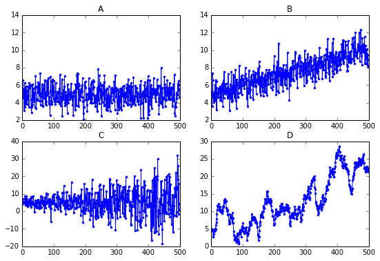
Answer:A This is white noise, which is stationary.
Seasonal Adjustment During Tax Season
Many time series exhibit strong seasonal behavior. The procedure for removing the seasonal component of a time series is called seasonal adjustment. For example, most economic data published by the government is seasonally adjusted.
You saw earlier that by taking first differences of a random walk, you get a stationary white noise process. For seasonal adjustments, instead of taking first differences, you will take differences with a lag corresponding to the periodicity.
Look again at the ACF of H&R Block's quarterly earnings, pre-loaded in the DataFrame HRB, and there is a clear seasonal component. The autocorrelation is high for lags 4,8,12,16,… because of the spike in earnings every four quarters during tax season. Apply a seasonal adjustment by taking the fourth difference (four represents the periodicity of the series). Then compute the autocorrelation of the transformed series.
Instructions:
- Create a new DataFrame of seasonally adjusted earnings by taking the lag-4 difference of quarterly earnings using the .diff() method.
- Examine the first 10 rows of the seasonally adjusted DataFrame and notice that the first four rows are NaN.
- Drop the NaN rows using the .dropna() method.
- Plot the autocorrelation function of the seasonally adjusted DataFrame.
from statsmodels.graphics.tsaplots import plot_acf
# Seasonally adjust quarterly earnings
HRBsa = HRB.diff(4)
# Print the first 10 rows of the seasonally adjusted series
print(HRBsa.head(10))
# Drop the NaN data in the first four rows
HRBsa = HRBsa.dropna()
# Plot the autocorrelation function of the seasonally adjusted series
plot_acf(HRBsa)
plt.show()

By seasonally adjusting the series, we eliminated the seasonal pattern in the autocorrelation function
Describe AR Model
Mathematical Description of AR(1) Model $$ R_t = \mu + \phi R_{t-1} + \epsilon_t $$
- Since only one lagged value or right hand side, this is called,
- AR model of order 1 or, AR(1) model
- AR paramter $\phi$
- For stationary $-1 < \phi < 1$
- Since only one lagged value or right hand side, this is called,
Interpretation of AR(1) Parameter
- Negative $\phi$: Mean Reversion
- Positive $\phi$: Momentum
High order AR Models
- AR(1) $$ R_t = \mu + \phi_1 R_{t-1} + \epsilon_t $$
- AR(2) $$ R_t = \mu + \phi_1 R_{t-1} + \phi_2 R_{t-2} + \epsilon_t $$
- AR(3) $$ R_t = \mu + \phi_1 R_{t-1} + \phi_2 R_{t-2} + \phi_3 R_{t-3} + \epsilon_t $$
- $\cdots$
Simulate AR(1) Time Series
You will simulate and plot a few AR(1) time series, each with a different parameter, $\phi$, using the arima_process module in statsmodels. In this exercise, you will look at an AR(1) model with a large positive $\phi$ and a large negative $\phi$, but feel free to play around with your own parameters.
There are a few conventions when using the arima_process module that require some explanation. First, these routines were made very generally to handle both AR and MA models. We will cover MA models next, so for now, just ignore the MA part. Second, when inputting the coefficients, you must include the zero-lag coefficient of 1, and the sign of the other coefficients is opposite what we have been using (to be consistent with the time series literature in signal processing). For example, for an AR(1) process with $\phi$=0.9, the array representing the AR parameters would be ar = np.array([1, -0.9])
Instructions:
- Import the class ArmaProcess in the arima_process module.
- Plot the simulated AR processes:
- Let ar1 represent an array of the AR parameters [1, ] as explained above. For now, the MA parameter array, ma1, will contain just the lag-zero coefficient of one.
- With parameters ar1 and ma1, create an instance of the class ArmaProcess(ar,ma) called AR_object1.
- Simulate 1000 data points from the object you just created, AR_object1, using the method .generate_sample(). Plot the simulated data in a subplot.
- Repeat for the other AR parameter.
from statsmodels.tsa.arima_process import ArmaProcess
# Plot 1: AR parameter = +0.9
plt.subplot(2,1,1)
ar1 = np.array([1, -0.9])
ma1 = np.array([1])
AR_object1 = ArmaProcess(ar1, ma1)
simulated_data_1 = AR_object1.generate_sample(nsample=1000)
plt.plot(simulated_data_1)
# Plot 2: AR parameter = -0.9
plt.subplot(2,1,2)
ar2 = np.array([1, 0.9])
ma2 = np.array([1])
AR_object2 = ArmaProcess(ar2, ma2)
simulated_data_2 = AR_object2.generate_sample(nsample=1000)
plt.plot(simulated_data_2)
plt.show()

The two AR parameters produce very different looking time series plots, but in the next exercise you'll really be able to distinguish the time series.
Compare the ACF for Several AR Time Series
The autocorrelation function decays exponentially for an AR time series at a rate of the AR parameter. For example, if the AR parameter, $\phi=+0.9$, the first-lag autocorrelation will be $0.9$, the second-lag will be $(0.9)^2=0.81$, the third-lag will be $(0.9)^3=0.729$, etc. A smaller AR parameter will have a steeper decay, and for a negative AR parameter, say $-0.9$, the decay will flip signs, so the first-lag autocorrelation will be $-0.9$, the second-lag will be $(−0.9)^2=0.81$, the third-lag will be $(−0.9)^3=−0.729$, etc.
The object simulated_data_1 is the simulated time series with an AR parameter of +0.9, simulated_data_2 is for an AR parameter of -0.9, and simulated_data_3 is for an AR parameter of 0.3
Instructions:
- Compute the autocorrelation function for each of the three simulated datasets using the plot_acf function with 20 lags (and suppress the confidence intervals by setting alpha=1).
ar3 = np.array([1, -0.3])
ma3 = np.array([1])
AR_object3 = ArmaProcess(ar3, ma3)
simulated_data_3 = AR_object3.generate_sample(nsample=1000)
from statsmodels.graphics.tsaplots import plot_acf
# Plot 1: AR parameter = +0.9
plot_acf(simulated_data_1, alpha=1, lags=20)
plt.show()
# Plot 2: AR parameter = -0.9
plot_acf(simulated_data_2, alpha=1, lags=20)
plt.show()
# Plot 3: AR parameter = +0.3
plot_acf(simulated_data_3, alpha=1, lags=20)
plt.show()


The ACF plots match what we predicted.
Match AR Model with ACF
Here are four Autocorrelation plots: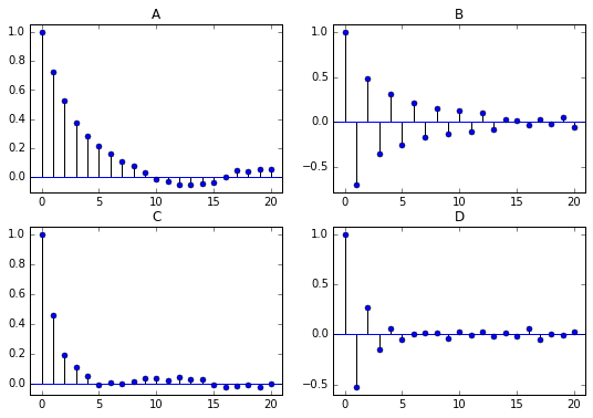 Which figure corresponds to an AR(1) model with an AR parameter of -0.5?
Answer:D
Estimating an AR Model
You will estimate the AR(1) parameter, $\phi$, of one of the simulated series that you generated in the earlier exercise. Since the parameters are known for a simulated series, it is a good way to understand the estimation routines before applying it to real data.
For simulated_data_1 with a true $\phi$ of 0.9, you will print out the estimate of $\phi$. In addition, you will also print out the entire output that is produced when you fit a time series, so you can get an idea of what other tests and summary statistics are available in statsmodels.
Instructions:
- Import the class ARMA in the module statsmodels.tsa.arima_model.
- Create an instance of the ARMA class called mod using the simulated data simulated_data_1 and the order (p,q) of the model (in this case, for an AR(1)), is order=(1,0).
- Fit the model mod using the method .fit() and save it in a results object called res.
- Print out the entire summary of results using the .summary() method.
- Just print out an estimate of the constant and $\phi$ using the .params attribute (no parentheses).
# from statsmodels.tsa.arima_model import ARMA
from statsmodels.tsa.arima.model import ARIMA
# Fit an AR(1) model to the first simulated data
mod = ARIMA(simulated_data_1, order=(1, 0,0))
res = mod.fit()
# Print out summary information on the fit
print(res.summary())
# Print out the estimate for the constant and for phi
print("When the true phi=0.9, the estimate of phi (and the constant) are:")
print(res.params)
Forecasting with an AR Model
In addition to estimating the parameters of a model that you did in the last exercise, you can also do forecasting, both in-sample and out-of-sample using statsmodels. The in-sample is a forecast of the next data point using the data up to that point, and the out-of-sample forecasts any number of data points in the future. These forecasts can be made using either the predict() method if you want the forecasts in the form of a series of data, or using the plot_predict() method if you want a plot of the forecasted data. You supply the starting point for forecasting and the ending point, which can be any number of data points after the data set ends.
For the simulated series simulated_data_1 with , you $\phi$ = 0.9 will plot in-sample and out-of-sample forecasts.
Instructions:
- Import the class ARMA in the module statsmodels.tsa.arima_model
- Create an instance of the ARMA class called mod using the simulated data simulated_data_1 and the order (p,q) of the model (in this case, for an AR(1) order=(1,0)
- Fit the model mod using the method .fit() and save it in a results object called res
- Plot the in-sample and out-of-sample forecasts of the data using the plot_predict() method
- Start the forecast 10 data points before the end of the 1000 point series at 990, and end the forecast 10 data points after the end of the series at point 1010
# from statsmodels.tsa.arima_model import ARMA
from statsmodels.tsa.arima.model import ARIMA
from statsmodels.graphics.tsaplots import plot_predict
# Forecast the first AR(1) model
# mod = ARMA(simulated_data_1, order=(1, 0))
mod = ARIMA(simulated_data_1, order=(1, 0,0))
res = mod.fit()
# res.plot_predict(start=990, end=1010)
plot_predict(res,dynamic=False)
plt.show()

import statsmodels
statsmodels.__version__
Let's Forecast Interest Rates
You will now use the forecasting techniques you learned in the last exercise and apply it to real data rather than simulated data. You will revisit a dataset from the first chapter:the annual data of 10-year interest rates going back 56 years, which is in a Series called interest_rate_data. Being able to forecast interest rates is of enormous importance, not only for bond investors but also for individuals like new homeowners who must decide between fixed and floating rate mortgages. You saw in the first chapter that there is some mean reversion in interest rates over long horizons. In other words, when interest rates are high, they tend to drop and when they are low, they tend to rise over time. Currently they are below long-term rates, so they are expected to rise, but an AR model attempts to quantify how much they are expected to rise.
Instructions:
- Import the class ARMA in the module statsmodels.tsa.arima_model.
- Create an instance of the ARMA class called mod using the annual interest rate data and choosing the order for an AR(1) model.
- Fit the model mod using the method .fit() and save it in a results object called res.
- Plot the in-sample and out-of-sample forecasts of the data using the .plot_predict() method.
- Pass the arguments start=0 to start the in-sample forecast from the beginning, and choose end to be '2022' to forecast several years in the future.
- Note that the end argument 2022 must be in quotes here since it represents a date and not an integer position.
bonds = pd.read_csv('./datasets/daily_rates.csv', index_col=0)
bonds.index = pd.to_datetime(bonds.index, format="%Y-%m-%d")
bonds.head()
interest_rate_data = bonds.resample(rule='A').last()
interest_rate_data.head()
from statsmodels.tsa.arima_model import ARMA
# Forecast interest rates using an AR(1) model
# mod = ARMA(interest_rate_data, order=(1, 0))
mod = ARIMA(interest_rate_data, order=(1, 0,0))
res = mod.fit()
# Plot the original series and the forecasted series
plot_predict(res,start=0, end='2022')
plt.legend(fontsize=8)
plt.show()

According to an AR(1) model, 10-year interest rates are forecasted to rise from 2.16%, towards the end of 2017 to 3.35% in five years.
Compare AR Model with Random Walk
Sometimes it is difficult to distinguish between a time series that is slightly mean reverting and a time series that does not mean revert at all, like a random walk. You will compare the ACF for the slightly mean-reverting interest rate series of the last exercise with a simulated random walk with the same number of observations.
You should notice when plotting the autocorrelation of these two series side-by-side that they look very similar.
Instructions:
- Import plot_acf function from the statsmodels module
- Create two axes for the two subplots
- Plot the autocorrelation function for 12 lags of the interest rate series interest_rate_data in the top plot
- Plot the autocorrelation function for 12 lags of the interest rate series simulated_data in the bottom plot
simulated_data = np.array([ 5. , 4.77522278, 5.60354317, 5.96406402, 5.97965372,
6.02771876, 5.5470751 , 5.19867084, 5.01867859, 5.50452928,
5.89293842, 4.6220103 , 5.06137835, 5.33377592, 5.09333293,
5.37389022, 4.9657092 , 5.57339283, 5.48431854, 4.68588587,
5.25218625, 4.34800798, 4.34544412, 4.72362568, 4.12582912,
3.54622069, 3.43999885, 3.77116252, 3.81727011, 4.35256176,
4.13664247, 3.8745768 , 4.01630403, 3.71276593, 3.55672457,
3.07062647, 3.45264414, 3.28123729, 3.39193866, 3.02947806,
3.88707349, 4.28776889, 3.47360734, 3.33260631, 3.09729579,
2.94652178, 3.50079273, 3.61020341, 4.23021143, 3.94289347,
3.58422345, 3.18253962, 3.26132564, 3.19777388, 3.43527681,
3.37204482])
from statsmodels.graphics.tsaplots import plot_acf
# Plot the interest rate series and the simulated random walk series side-by-side
fig, axes = plt.subplots(2, 1)
# Plot the autocorrelation of the interest rate series in the top plot
fig = plot_acf(interest_rate_data, alpha=1, lags=12, ax=axes[0]);
# Plot the autocorrelation of the simulated random walk series in the bottom plot
fig = plot_acf(simulated_data, alpha=1, lags=12, ax=axes[1]);
# Label axes
axes[0].set_title("Interest Rate Data");
axes[1].set_title("Simulated Random Walk Data");
plt.show()

Notice the Autocorrelation functions look very similar for the two series.
Choosing the Right Model
- Identifying the Order of an AR Model
- The order of an AR(p) model will usually be unknown
- Two techniques to determine order
- Partial Autocorrelation Funciton
- Information criteria
- Partial Autocorrelation Function (PACF) $$ \begin{aligned} R_t &= \phi_{0,1} + \color{red}{\phi_{1,1}} R_{t-1} + \epsilon_{1t} \\ R_t &= \phi_{0,2} + \phi_{1,2} R_{t-1} + \color{red}{\phi_{2,2}} R_{t-2} + \epsilon_{2t} \\ R_t &= \phi_{0,3} + \phi_{1,3} R_{t-1} + \phi_{2,3} R_{t-2} + \color{red}{\phi_{3,3}} R_{t-3} + \epsilon_{3t} \\ R_t &= \phi_{0,4} + \phi_{1,4} R_{t-1} + \phi_{2,4} R_{t-2} + \phi_{3,4} R_{t-3} + \color{red}{\phi_{4,4}} R_{t-4} + \epsilon_{4t} \\ \end{aligned} $$
- Information Criteria
- Information criteria: adjusts goodness-of-fit for number of parameters
- Two popular adjusted goodness-of-fit measures
Estimate Order of Model PACF
One useful tool to identify the order of an AR model is to look at the Partial Autocorrelation Function (PACF). In this exercise, you will simulate two time series, an AR(1) and an AR(2), and calculate the sample PACF for each. You will notice that for an AR(1), the PACF should have a significant lag-1 value, and roughly zeros after that. And for an AR(2), the sample PACF should have significant lag-1 and lag-2 values, and zeros after that.
Just like you used the plot_acf function in earlier exercises, here you will use a function called plot_pacf in the statsmodels module.
Instructions:
- Import the modules for simulating data and for plotting the PACF
- Simulate an AR(1) with $\phi$=0.6 (remember that the sign for the AR parameter is reversed)
- Plot the PACF for simulated_data_1 using the
plot_pacffunction - Simulate an AR(2) with $\phi _1$ = 0.6, $\phi _2$ = 0.3 (again, reverse the signs)
- Plot the PACF for simulated_data_2 using the
plot_pacffunction
from statsmodels.graphics.tsaplots import plot_pacf
from statsmodels.tsa.arima_process import ArmaProcess
# Simulate AR(1) with phi=+0.6
ma = np.array([1])
ar = np.array([1, -0.6])
AR_object = ArmaProcess(ar, ma)
simulated_data_1 = AR_object.generate_sample(nsample=5000)
# Plot PACF for AR(1)
plot_pacf(simulated_data_1, lags=20)
plt.show()
# simulated AR(2) with phi1=+0.6, phi2=+0.3
ma = np.array([1])
ar = np.array([1, -0.6, -0.3])
AR_object = ArmaProcess(ar, ma)
simulated_data_2 = AR_object.generate_sample(nsample=5000)
# Plot PACF for AR(2)
plot_pacf(simulated_data_2, lags=20)
plt.show()


Notice that the number of significant lags for the PACF indicate the order of the AR model
Estimate Order of Model:Information Criteria
Another tool to identify the order of a model is to look at the Akaike Information Criterion (AIC) and the Bayesian Information Criterion (BIC). These measures compute the goodness of fit with the estimated parameters, but apply a penalty function on the number of parameters in the model. You will take the AR(2) simulated data from the last exercise, saved as simulated_data_2, and compute the BIC as you vary the order, p, in an AR(p) from 0 to 6.
Instructions:
- Import the ARMA module for estimating the parameters and computing BIC.
- Initialize a numpy array BIC, which we will use to store the BIC for each AR(p) model.
- Loop through order p for p = 0,…,6.
- For each p, fit the data to an AR model of order p.
- For each p, save the value of BIC using the .bic attribute (no parentheses) of res.
- Plot BIC as a function of p (for the plot, skip p=0 and plot for p=1,…6).
from statsmodels.tsa.arima.model import ARIMA
# Fit the data to an AR(p) for p = 0,...,6 , and save the BIC
BIC = np.zeros(7)
for p in range(7):
mod = ARIMA(simulated_data_2, order=(p, 0,0))
res = mod.fit()
# Save BIC for AR(p)
BIC[p] = res.bic
# Plot the BIC as a function of p
plt.plot(range(1,7), BIC[1:7], marker='o')
plt.xlabel('Order of AR Model')
plt.ylabel('Bayesian Information Criterion')
plt.show()

For an AR(2), the BIC achieves its minimum at p=2, which is what we expect.
Simulate MA(1) Time Series
You will simulate and plot a few MA(1) time series, each with a different parameter, , using the arima_process module in statsmodels, just as you did in the last chapter for AR(1) models. You will look at an MA(1) model with a large positive $\theta$ and a large negative .
As in the last chapter, when inputting the coefficients, you must include the zero-lag coefficient of 1, but unlike the last chapter on AR models, the sign of the MA coefficients is what we would expect. For example, for an MA(1) process with $\theta$ = -0.9, the array representing the MA parameters would be ma = np.array([1, -0.9])
Instructions:
- Import the class ArmaProcess in the arima_process module.
- Plot the simulated MA(1) processes
- Let ma1 represent an array of the MA parameters [1, $\theta$] as explained above. The AR parameter array will contain just the lag-zero coefficient of one.
- With parameters ar1 and ma1, create an instance of the class ArmaProcess(ar,ma) called MA_object1.
- Simulate 1000 data points from the object you just created, MA_object1, using the method .generate_sample(). Plot the simulated data in a subplot.
- Repeat for the other MA parameter.
from statsmodels.tsa.arima_process import ArmaProcess
# Plot 1: MA parameter = -0.9
plt.subplot(2, 1, 1)
ar1 = np.array([1])
ma1 = np.array([1, -0.9])
MA_object1 = ArmaProcess(ar1, ma1)
simulated_data_1 = MA_object1.generate_sample(nsample=1000)
plt.plot(simulated_data_1)
plt.show()
# Plot 2: MA parameter: +0.9
plt.subplot(2, 1, 2)
ar2 = np.array([1])
ma2 = np.array([1, 0.9])
MA_object2 = ArmaProcess(ar2, ma2)
simulated_data_2 = MA_object2.generate_sample(nsample=1000)
plt.plot(simulated_data_2)
plt.show()


The two MA parameters produce different time series plots, but in the next exercise you'll really be able to distinguish the time series.
Compute the ACF for Several MA Time Series
Unlike an AR(1), an MA(1) model has no autocorrelation beyond lag 1, an MA(2) model has no autocorrelation beyond lag 2, etc. The lag-1 autocorrelation for an MA(1) model is not $\theta$, but rather $\frac{\theta}{1+\theta^2}$. For example, if the MA parameter, $\theta$, is = +0.9, the first-lag autocorrelation will be $\frac{0.9}{1 + (0.9)^2} = 0.497$, and the autocorrelation at all other lags will be zero. If the MA parameter, $\theta$, is -0.9, the first-lag autocorrelation will be $\frac{-0.9}{1 + (-0.9)^2}$ = -0.497.
You will verify these autocorrelation functions for the three time series you generated in the last exercise.
Instructions:
- simulated_data_1 is the first simulated time series with an MA parameter of $\theta = -0.9$ .
- Compute the autocorrelation function of simulated_data_1 using the plot_acf function with 20 lags.
ar3 = np.array([1])
ma3 = np.array([1, -0.3])
MA_object3 = ArmaProcess(ar3, ma3)
simulated_data_3 = MA_object3.generate_sample(nsample=1000)
from statsmodels.graphics.tsaplots import plot_acf
# Plot 1: MA parameter = -0.9
plot_acf(simulated_data_1, lags=20)
plt.show()

- simulated_data_2 is the second simulated time series with an MA parameter of $\theta = 0.9$.
- Compute the autocorrelation function using the plot_acf function with lags=20
plot_acf(simulated_data_2, lags=20)
plt.show()

- simulated_data_3 is the third simulated time series with an MA parameter of $\theta= - 0.3$.
- Compute the autocorrelation function using the plot_acf() function with 20 lags.
plot_acf(simulated_data_3, lags=20)
plt.show()

The ACF plots match what we predicted.
Match ACF with MA Model
Here are four Autocorrelation plots: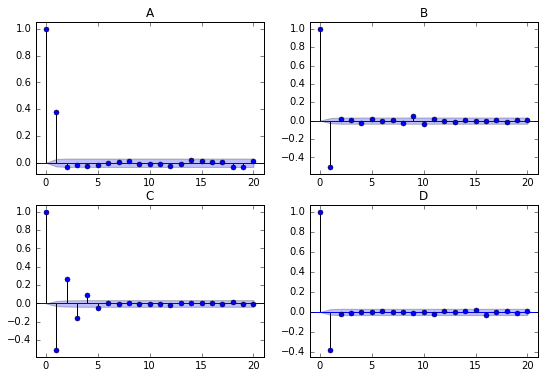
Which figure corresponds to an MA(1) model with an MA parameter of -0.5
Ans:D
Estimating an MA Model
You will estimate the MA(1) parameter, $\theta$, of one of the simulated series that you generated in the earlier exercise. Since the parameters are known for a simulated series, it is a good way to understand the estimation routines before applying it to real data.
For simulated_data_1 with a true $\theta$ of -0.9, you will print out the estimate of $\theta$. In addition, you will also print out the entire output that is produced when you fit a time series, so you can get an idea of what other tests and summary statistics are available in statsmodels.
Instructions:
- Import the class ARMA in the module statsmodels.tsa.arima_model.
- Create an instance of the ARMA class called mod using the simulated data simulated_data_1 and the order (p,q) of the model (in this case, for an MA(1)), is order=(0,1).
- Fit the model mod using the method .fit() and save it in a results object called res.
- Print out the entire summary of results using the .summary() method.
- Just print out an estimate of the constant and theta parameter using the .params attribute (no arguments).
from statsmodels.tsa.arima_model import ARMA
# Fit an MA(1) model to the first simulated data
# mod = ARMA(simulated_data_1, order=(0, 1))
mod = ARIMA(simulated_data_1, order=(0, 0, 1))
res = mod.fit()
# Print out summary information on the fit
print(res.summary())
# Print out the estimate for the constant and for theta
print("When the true theta=-0.9, the estimate of theta (and the constant) are:")
print(res.params)
Forecasting with MA Model
As you did with AR models, you will use MA models to forecast in-sample and out-of-sample data using the plot_predict() function in statsmodels.
For the simulated series simulated_data_1 with $\theta=−0.9$, you will plot in-sample and out-of-sample forecasts. One big difference you will see between out-of-sample forecasts with an MA(1) model and an AR(1) model is that the MA(1) forecasts more than one period in the future are simply the mean of the sample.
Instructions:
- Import the class ARIMA and also import the function plot_predict
- Create an instance of the ARIMA class called mod using the simulated data simulated_data_1 and the (p,d,q) order of the model (in this case, for an MA(1)), order=(0,0,1)
- Fit the model mod using the method .fit() and save it in a results object called res
- Plot the in-sample data starting with data point 950
- Plot out-of-sample forecasts of the data and confidence intervals using the plot_predict() function, starting with data point 950 and ending the forecast at point 1010
from statsmodels.tsa.arima.model import ARIMA
# Forecast the first MA(1) model
mod = ARIMA(simulated_data_1, order=(0,0,1))
res = mod.fit()
plot_predict(res,start=1000, end=1010)
plt.show()

plot_predict(res, start=990, end=1010);

ARMA models
ARMA(1,1) model: $$ R_t = \mu + \phi R_{t-1} + \epsilon_t + \theta \epsilon_{t-1} $$
Converting Between ARMA, AR, and MA Models
- Converting AR(1) into an MA($\infty$) $$ \begin{aligned} R_t &= \mu + \phi R_{t-1} + \epsilon_t \\ R_t &= \mu + \phi( \mu + \phi R_{t-2} + \epsilon_{t-1}) + \epsilon_t \\ &\vdots \\ R_t &= \frac{\mu}{1-\phi} + \epsilon_t + \phi \epsilon_{t-1} - \phi^2 \epsilon_{t-2} + \phi^3 \epsilon_{t-3} + \dots \end{aligned} $$
High Frequency Stock Prices
Higher frequency stock data is well modeled by an MA(1) process, so it's a nice application of the models in this chapter.
The DataFrame intraday contains one day's prices (on September 1, 2017) for Sprint stock (ticker symbol "S") sampled at a frequency of one minute. The stock market is open for 6.5 hours (390 minutes), from 9:30am to 4:00pm.
Before you can analyze the time series data, you will have to clean it up a little, which you will do in this and the next two exercises. When you look at the first few rows (see the IPython Shell), you'll notice several things. First, there are no column headers.The data is not time stamped from 9:30 to 4:00, but rather goes from 0 to 390. And you will notice that the first date is the odd-looking "a1504272600". The number after the "a" is Unix time which is the number of seconds since January 1, 1970. This is how this dataset separates each day of intraday data.
If you look at the data types, you'll notice that the DATE column is an object, which here means a string. You will need to change that to numeric before you can clean up some missing data.
The source of the minute data is Google Finance (see here on how the data was downloaded).
Instructions:
- Manually change the first date to zero using .iloc[0,0].
- Change the two column headers to 'DATE' and 'CLOSE' by setting intraday.columns equal to a list containing those two strings.
- Use the pandas attribute .dtypes (no parentheses) to see what type of data are in each column.
- Convert the 'DATE' column to numeric using the pandas function to_numeric().
- Make the 'DATE' column the new index of intraday by using the pandas method .set_index(), which will take the string 'DATE' as its argument (not the entire column, just the name of the column).
intraday = pd.read_csv('./datasets/Sprint_Intraday.txt', header=None)
intraday = intraday.loc[:, :1]
intraday.head()
import datetime
# Change the first date to zero
intraday.iloc[0, 0] = 0
# Change the column headers to 'DATE' and 'CLOSE'
intraday.columns = ['DATE', 'CLOSE']
# Examine the data types for each column
print(intraday.dtypes)
# Convert DATE column to numeric
intraday['DATE'] = pd.to_numeric(intraday['DATE'])
# Make the 'DATE' column the new index
intraday = intraday.set_index('DATE')
More Data Cleaning:Missing Data
When you print out the length of the DataFrame intraday, you will notice that a few rows are missing. There will be missing data if there are no trades in a particular one-minute interval. One way to see which rows are missing is to take the difference of two sets: the full set of every minute and the set of the DataFrame index which contains missing rows. After filling in the missing rows, you can convert the index to time of day and then plot the data.
Stocks trade at discrete one-cent increments (although a small percentage of trades occur in between the one-cent increments) rather than at continuous prices, and when you plot the data you should observe that there are long periods when the stock bounces back and forth over a one cent range. This is sometimes referred to as "bid/ask bounce".
Instructions:
- Print out the length of intraday using len()
- Find the missing rows by making range(391) into a set and then subtracting the set of the intraday index, intraday.index.
- Fill in the missing rows using the .reindex() method, setting the index equal to the full range(391) and forward filling the missing data by setting the method argument to 'ffill'.
- Change the index to times using pandas function date_range(), starting with '2017-09-01 9:30' and ending with '2017-09-01 16:00' and passing the argument freq='1min'.
- Plot the data and include gridlines.
print("If there were no missing rows, there would be 391 rows of minute data")
print("The actual length of the DataFrame is:", len(intraday))
# Everything
set_everything = set(range(391))
# The intraday index as a set
set_intraday = set(intraday.index)
# Calculate the difference
set_missing = set_everything - set_intraday
# Print the difference
print("Missing rows: ", set_missing)
# Fill in the missing rows
intraday = intraday.reindex(range(391), method='ffill')
# Change the index to the intraday times
intraday.index = pd.date_range(start='2017-09-01 9:30', end='2017-09-01 16:00', freq='1min')
# Plot the intraday time series
intraday.plot(grid=True)

Missing data is common with high frequency financial time series, so good job fixing that.
Applying an MA Model
The bouncing of the stock price between bid and ask induces a negative first order autocorrelation, but no autocorrelations at lags higher than 1. You get the same ACF pattern with an MA(1) model. Therefore, you will fit an MA(1) model to the intraday stock data from the last exercise.
The first step is to compute minute-by-minute returns from the prices in intraday, and plot the autocorrelation function. You should observe that the ACF looks like that for an MA(1) process. Then, fit the data to an MA(1), the same way you did for simulated data.
Instructions:
- Import plot_acf and ARMA modules from statsmodels
- Compute minute-to-minute returns from prices:
- Compute returns with the .pct_change() method
- Use the pandas method .dropna() to drop the first row of returns, which is NaN
- Plot the ACF function with lags up to 60 minutes
- Fit the returns data to an MA(1) model and print out the MA(1) parameter
from statsmodels.graphics.tsaplots import plot_acf
from statsmodels.tsa.arima_model import ARMA
# Compute returns from prices and drop the NaN
returns = intraday.pct_change()
returns = returns.dropna()
# Plot ACF of returns with lags up to 60 minutes
plot_acf(returns, lags=60)
plt.show()
# fit the data to an MA(1) model
# mod = ARMA(returns, order=(0, 1))
mod = ARIMA(returns, order=(0, 0, 1))
res = mod.fit()
print(res.params)

Equivalence of AR(1) and MA(infinity)
To better understand the relationship between MA models and AR models, you will demonstrate that an AR(1) model is equivalent to an MA($\infty$) model with the appropriate parameters.
You will simulate an MA model with parameters $0.8,0.8^2,0.8^3,\cdots$ for a large number (30) lags and show that it has the same Autocorrelation Function as an AR(1) model with $\phi=0.8$.
Note, to raise a number x to the power of an exponent n, use the format x**n.
Instructions:
- Import the modules for simulating data and plotting the ACF from statsmodels
- Use a list comprehension to build a list with exponentially decaying MA parameters:
- Simulate 5000 observations of the MA(30) model
- Plot the ACF of the simulated series
from statsmodels.tsa.arima_process import ArmaProcess
from statsmodels.graphics.tsaplots import plot_acf
# Build a list MA parameters
ma = [0.8 ** i for i in range(30)]
# Simulate the MA(30) model
ar = np.array([1])
AR_object = ArmaProcess(ar, ma)
simulated_data = AR_object.generate_sample(nsample=5000)
# Plot the ACF
plot_acf(simulated_data, lags=30)
plt.show()

Notice that the ACF looks the same as an AR(1) with parameter 0.8
Putting It All Together
This chapter will show you how to model two series jointly using cointegration models. Then you'll wrap up with a case study where you look at a time series of temperature data from New York City.
Cointegration Models
- What is Cointegration?
- Two series, $P_t$ and $Q_t$ can be random walks
- But the linear combination $P_t - c Q_t$ may not be a random walk!
- If that's true
- $P_t - c Q_t$ is forecastable
- $P_t$ and $Q_t$ are said to be cointegrated
- Analogy:Dog on a Leash - $P_t =$ Owner
- $Q_t =$ Dog
- Both series look like a random walk
- Difference of distance between them, looks mean reverting
- If dog falls too far behind, it gets pulled forward
- If dog gets too far ahead, it gets pulled back
- What types of series are cointegrated?
- Economic substitutes
- Heating Oil and Natural Gas
- Platinum and Palladium
- Corn and Wheat
- Corn and Sugar
- $\dots$
- Bitcoin and Ethereum
- Economic substitutes
- Two steps to test for Cointegration
- Regress $P_t$ on$Q_t$ and get slope $c$
- Run Augmented Dickey-Fuller test on $P_t - c Q_t$ to test for random walk
- Alternatively, can use
cointfunction in statsmodels that combines both steps
A Dog on a Leash? (Part 1)
The Heating Oil and Natural Gas prices are pre-loaded in DataFrames HO and NG. First, plot both price series, which look like random walks. Then plot the difference between the two series, which should look more like a mean reverting series (to put the two series in the same units, we multiply the heating oil prices, in $/gallon, by 7.25, which converts it to $/millionBTU, which is the same units as Natural Gas).
The data for continuous futures (each contract has to be spliced together in a continuous series as contracts expire) was obtained from Quandl.
Instructions:
- Plot Heating Oil, HO, and Natural Gas, NG, on the same subplot
- Make sure you multiply the HO price by 7.25 to match the units of NG
- Plot the spread on a second subplot
- The spread will be 7.25*HO - NG
HO = pd.read_csv('./datasets/CME_HO1.csv', index_col=0)
NG = pd.read_csv('./datasets/CME_NG1.csv', index_col=0)
HO.index = pd.to_datetime(HO.index, format='%m/%d/%Y')
NG.index = pd.to_datetime(NG.index, format='%m/%d/%Y')
HO = HO.sort_index()
NG = NG.sort_index()
HO.head()
NG.head()
plt.subplot(2, 1, 1)
plt.plot(7.25 * HO, label='Heating Oil')
plt.plot(NG, label='Natural Gas')
plt.legend(loc='best', fontsize='small')
# Plot the spread
plt.subplot(2, 1, 2)
plt.plot(7.25 * HO - NG, label='Spread')
plt.legend(loc='best', fontsize='small')
plt.axhline(y=0, linestyle='--', color='k')
plt.show()

Notice from the plot that when Heating Oil briefly dipped below Natural Gas, it quickly reverted back up.
A Dog on a Leash? (Part 2)
To verify that Heating Oil and Natural Gas prices are cointegrated, First apply the Dickey-Fuller test separately to show they are random walks. Then apply the test to the difference, which should strongly reject the random walk hypothesis. The Heating Oil and Natural Gas prices are pre-loaded in DataFrames HO and NG.
Instructions:
- Perform the adfuller test on HO and on NG separately, and save the results (results are a list)
- The argument for adfuller must be a series, so you need to include the column 'Close'
- Print just the p-value (item [1] in the list)
- Do the same thing for the spread, again converting the units of HO, and using the column 'Close' of each DataFrame
from statsmodels.tsa.stattools import adfuller
# Compute the ADF for HO and NG
result_HO = adfuller(HO['Close'])
print("The p-value for the ADF test on HO is ", result_HO[1])
result_NG = adfuller(NG['Close'])
print("The p-value for the ADF test on NG is ", result_NG[1])
# Compute the ADF of the spread
result_spread = adfuller(7.25 * HO['Close'] - NG['Close'])
print("The p-value for the ADF test on the spread is ", result_spread[1])
As we expected, we cannot reject the hypothesis that the individual futures are random walks, but we can reject that the spread is a random walk.
Are Bitcoin and Ethereum Cointegrated?
Cointegration involves two steps:regressing one time series on the other to get the cointegration vector, and then perform an ADF test on the residuals of the regression. In the last example, there was no need to perform the first step since we implicitly assumed the cointegration vector was (1,−1). In other words, we took the difference between the two series (after doing a units conversion). Here, you will do both steps. You will regress the value of one cryptocurrency, bitcoin (BTC), on another cryptocurrency, ethereum (ETH). If we call the regression coefficient b, then the cointegration vector is simply (1,−b). Then perform the ADF test on BTC −b ETH.
BTC = pd.read_csv('./datasets/BTC.csv', index_col='Date', parse_dates=['Date'])
ETH = pd.read_csv('./datasets/ETH.csv', index_col='Date', parse_dates=['Date'])
BTC.head()
import statsmodels.api as sm
from statsmodels.tsa.stattools import adfuller
# Regress BTC on ETH
ETH = sm.add_constant(ETH)
result = sm.OLS(BTC, ETH).fit()
# Compare ADF
b = result.params[1]
adf_stats = adfuller(BTC['Price'] - b * ETH['Price'])
print("The p-value for the ADF test is ", adf_stats[1])
The data suggests that Bitcoin and Ethereum are cointegrated.
Is Temperature a Random Walk (with Drift)?
An ARMA model is a simplistic approach to forecasting climate changes, but it illustrates many of the topics covered in this class.
The DataFrame temp_NY contains the average annual temperature in Central Park, NY from 1870-2016 (the data was downloaded from the NOAA here). Plot the data and test whether it follows a random walk (with drift).
Instructions:
- Convert the index of years into a datetime object using pd.to_datetime(), and since the data is annual, pass the argument format='%Y'.
- Plot the data using .plot()
- Compute the p-value the Augmented Dickey Fuller test using the adfuller function.
- Save the results of the ADF test in result, and print out the p-value in result[1].
temp_NY = pd.read_csv('./datasets/NOAA_TAVG.csv', index_col=0)
temp_NY.index = pd.to_datetime(temp_NY.index, format='%Y')
temp_NY.head()
temp_NY.plot()
# Compute and print ADF p-value
result = adfuller(temp_NY['TAVG'])
print("The p-value for the ADF test is ", result[1])

The data seems to follow a random walk with drift.
Getting "Warmed" Up:Look at Autocorrelations
Since the temperature series, temp_NY, is a random walk with drift, take first differences to make it stationary. Then compute the sample ACF and PACF. This will provide some guidance on the order of the model.
Instructions:
- Import the modules for plotting the sample ACF and PACF
- Take first differences of the DataFrame temp_NY using the pandas method .diff()
- Create two subplots for plotting the ACF and PACF
- Plot the sample ACF of the differenced series
- Plot the sample PACF of the differenced series
from statsmodels.graphics.tsaplots import plot_acf, plot_pacf
# Take first difference of the temperature Series
chg_temp = temp_NY.diff()
chg_temp = chg_temp.dropna()
# Plot the ACF and PACF on the same page
fig, axes = plt.subplots(2, 1)
# Plot the ACF
plot_acf(chg_temp, lags=20, ax=axes[0])
# Plot the PACF
plot_pacf(chg_temp, lags=20, ax=axes[1])
plt.show()

There is no clear pattern in the ACF and PACF except the negative lag-1 autocorrelation in the ACF.
Which ARMA Model is Best?
Recall from Chapter 3 that the Akaike Information Criterion (AIC) can be used to compare models with different numbers of parameters. It measures goodness-of-fit, but places a penalty on models with more parameters to discourage overfitting. Lower AIC scores are better.
Fit the temperature data to an AR(1), AR(2), and ARMA(1,1) and see which model is the best fit, using the AIC criterion. The AR(2) and ARMA(1,1) models have one more parameter than the AR(1) has.
The annual change in temperature is in a DataFrame chg_temp.
Instructions:
- For each ARMA model, create an instance of the ARMA class, passing the data and the order=(p,q). p is the autoregressive order; q is the moving average order.
- Fit the model using the method .fit().
- Print the AIC value, found in the .aic element of the results.
NOTE: Older Version
# Import the module for estimating an ARMA model
from statsmodels.tsa.arima_model import ARMA
# Fit the data to an AR(1) model and print AIC:
mod_ar1 = ARMA(chg_temp, order=(1, 0))
res_ar1 = mod_ar1.fit()
print("The AIC for an AR(1) is: ", res_ar1.aic)
# Fit the data to an AR(2) model and print AIC
mod_ar2 = ARMA(chg_temp, order=(2, 0))
res_ar2 = mod_ar2.fit()
print("The AIC for an AR(2) is: ", res_ar2.aic)
# fit the data to an ARMA(1, 1) model and print AIC
mod_arma11 = ARMA(chg_temp, order=(1, 1))
res_arma11 = mod_arma11.fit()
print("The AIC for an ARMA(1,1) is: ", res_arma11.aic)
<script.py> output:
The AIC for an AR(1) is: 510.534689831391
The AIC for an AR(2) is: 501.9274123160228
The AIC for an ARMA(1,1) is: 469.07291479787045
from statsmodels.tsa.arima.model import ARIMA
# Fit the data to an AR(1) model and print AIC:
mod_ar1 = ARIMA(chg_temp, order=(1, 0,0))
res_ar1 = mod_ar1.fit()
print("The AIC for an AR(1) is: ", res_ar1.aic)
# Fit the data to an AR(2) model and print AIC
mod_ar2 = ARIMA(chg_temp, order=(2, 0, 0))
res_ar2 = mod_ar2.fit()
print("The AIC for an AR(2) is: ", res_ar2.aic)
# fit the data to an ARMA(1, 1) model and print AIC
mod_arma11 = ARIMA(chg_temp, order=(1, 1,0))
res_arma11 = mod_arma11.fit()
print("The AIC for an ARMA(1,1) is: ", res_arma11.aic)
Don't Throw Out That Winter Coat Yet
Finally, you will forecast the temperature over the next 30 years using an ARMA(1,1) model, including confidence bands around that estimate. Keep in mind that the estimate of the drift will have a much bigger impact on long range forecasts than the ARMA parameters.
Earlier, you determined that the temperature data follows a random walk and you looked at first differencing the data. In this exercise, you will use the ARIMA module on the temperature data (before differencing), which is identical to using the ARMA module on changes in temperature, followed by taking cumulative sums of these changes to get the temperature forecast.
The data is preloaded in a DataFrame called temp_NY.
Instructions:
- Create an instance of the ARIMA class called mod for an integrated ARMA(1,1) model
- The d in order(p,d,q) is one, since we first differenced once
- Fit mod using the .fit() method and call the results res
- Forecast the series using the plot_predict() method on res
- Choose the start date as 1872-01-01 and the end date as 2046-01-01
Older Version Code:
# Import the ARIMA module from statsmodels
from statsmodels.tsa.arima_model import ARIMA
# Forecast temperatures using an ARIMA(1,1,1) model
mod = ARIMA(temp_NY, order=(1,1,1))
res = mod.fit()
# Plot the original series and the forecasted series
res.plot_predict(start='1872-01-01', end='2046-01-01')
plt.show()
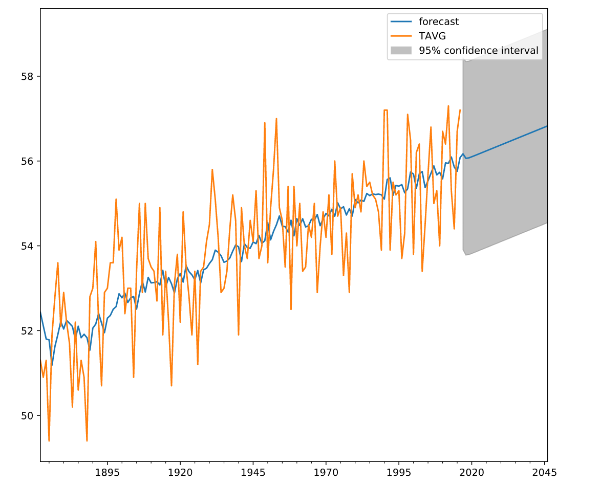
According to the model, the temperature is expected to be about 0.6 degrees higher in 30 years (almost entirely due to the trend), but the 95% confidence interval around that is over 5 degrees.
from statsmodels.tsa.arima.model import ARIMA
from statsmodels.graphics.tsaplots import plot_predict
# Forecast temperatures using an ARIMA(1,1,1) model
mod = ARIMA(temp_NY, order=(1,1,1))
res = mod.fit()
# Plot the original series and the forecasted series
plot_predict(res, start='1872', end='2046')
plt.show()

According to the model, the temperature is expected to be about 0.6 degrees higher in 30 years (almost entirely due to the trend), but the 95% confidence interval around that is over 5 degrees.